
|
This article originally appeared in Geospatial Solutions Magazine's Net Results column of July 1, 2003. Other Net Results articles about the role of emerging technologies in the exchange of spatial information are also online. |
| 1. Introduction and Glossary 2. Naive to cynical 3. Cynical to critical 4. Pure Critics | |
| A break between cynical and critical One of the many rest stops while climbing up the learning curve of ESDA is a review of spatial autocorrelation. An example from an Indonesian coral reef helps clarify the concept: Healthy coral reefs support highly heterogeneous species populations. Pollution, typically muddy runoff from shoreline construction, can clog and kill the coral, turning the damaged reef into a homogeneous algae farm. Comparing one area of a healthy reef to its neighbors should show little similarity, whereas any spot in a dead reef will be similar to any other spot — algae everywhere. Marine conservationists want to track the spread of reef damage in order to apply realistic management schemes. High spectral resolution data can discriminate between healthy corals, bleached corals, sea grass and algae-covered surfaces, but sensors capable of this resolution are not available from a satellite platform. Less-detailed data, such as SPOT (www.spot.com) HRV or Landsat TM imagery are available, however. So, rather than attempting to detect change in species mix over time, why not compare change in diversity over time instead? This is where spatial autocorrelation helps. Although too coarse (at 20- or 30-meter pixel resolution) to reveal specific species, SPOT and Landsat data pixels will either be similar to their neighbors or different. Such was the approach Heather Holden (National University of Singapore), Chris Derksen, and Ellsworth LeDrew (University of Waterloo, Canada) took to detect change in the Bunaken National Marine Park, North Sulawesi, Indonesia (www.gisdevelopment.net/aars/acrs/2000/ts3/cost006.shtml). In light of this change detection example, the reef researchers’ definition of spatial autocorrelation should make sense: “Spatial autocorrelation is…the situation where one variable (reflectance value of a pixel in this case) is related to another variable located nearby (surrounding pixels). Spatial autocorrelation is useful since it not only considers the value of that pixel (magnitude of reflectance), but also the relationship between that pixel and its surrounding pixels.” Said another way, spatial autocorrelation reveals spatial patterns in which areas (or points) close together are more similar than areas (or points) that are far apart. Zero to sixty. This is the basic ESDA concept; now try leaping the gap to explore one of its details. As CSISS’s Sam Ying points out when recounting the history of spatial autocorrelation (www.csiss.org/classics/content/61), it is scale dependent. Ying illustrates his point with two identical datasets, the first divided into four squares in which the squares adjacent to white squares are always black, displaying no spatial autocorrelation. The second, though containing identical underlying data, is divided into 16 grid cells, resulting in positive spatial autocorrelation: the squares in the corners are surrounded on two sides with squares of the same color (see Figure 2). |
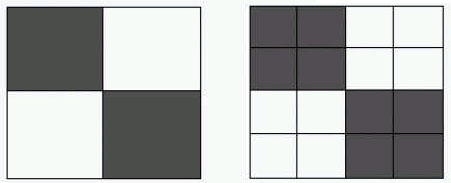
Figure 3: Identical datasets (each with two white areas and two black areas) can return different spatial autocorrelation results. The left, more coarse grid has no spatial autocorrelation. The right, finer grid does register spatial autocorrelation — clusters of similarity in the corners of its extent. |
| Another consideration — what if the “grid” was irregular, as with census polygons? Comparing a cell to its neighbors can result in an unbalanced connectedness structure if the neighboring polygons have very different areas. For instance, smaller units tend to have many neighbors while larger ones have very few or none at all (islands). In this case, an alternative approach (such as “K-nearest neighbors”) might be prudent. Quantifying how spatial autocorrelation changes at different scales or when spatial units have very different areas, and how it might change the results of a study such as coral reef change detection, is where the painful (or exciting) mathematics enter the picture, and where overwhelmed novice spatial experts defer to statisticians. |
| 1. Introduction and Glossary 2. Naive to cynical 3. Cynical to critical 4. Pure Critics |
|
|